This toot from Charlie Gao about the new release of {mirai} (R’s newest async evaluation framework) mentions the new function race_mirai() which
returns as soon as the first mirai you pass to it resolves. This supports more async usage patterns in #RStats.
This caught my attention, partly because I’ve been thinking about “alternate pathway” designs recently, albeit in a very different context.
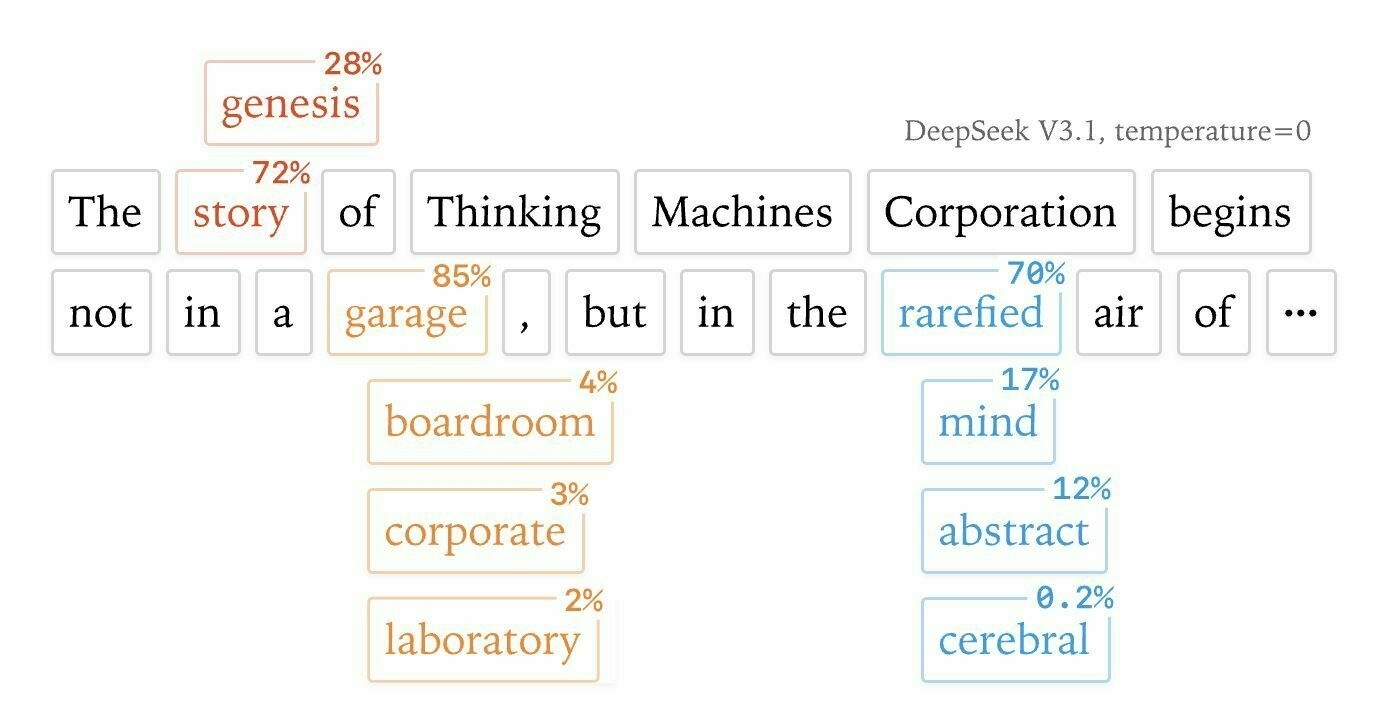
I saw the latest paper from Thinking Machines Lab titled ‘Defeating Nondeterminism in LLM Inference’ and the header “image” (actually a complex svg, not a rasterised image) for that shows the result of an LLM annotated with alternatives which were not selected (but might have been with higher temperature) and their ‘score’ for how likely they were to be selected (presumably)
This reminded me of Tufte’s graphical sentences, apparently in his book ‘Seeing with Fresh Eyes’ but which I could only find one blog post referencing

I think it’s an interesting idea, and I posted on LinkedIn as such but didn’t get much of a response about it.
Sometimes there are multiple options that fit at a given point, and we need to choose one based on some criteria. In the LLM space it’s “what word best looks like a good answer?”, but in programming we sometimes need to ask “what algorithm has the best performance for this calculation?”
Back to {mirai} - the example given was two functions m1() and m2() which sleep for 0.2s and 0.1s, respectively. Passing a list of these to race_mirai() and wrapped with some timing code, it’s clear that each time it’s run, the value is returned after the 0.1s evaluation has taken place.
library(mirai)

daemons(2)
m1 <- mirai(Sys.sleep(0.2))
m2 <- mirai(Sys.sleep(0.1))
start <- Sys.time()
race_mirai(list(m1, m2))
Sys.time() - start
#> Time difference of 0.105644 secs
race_mirai(list(m1, m2))
Sys.time() - start
#> Time difference of 0.2042089 secs
daemons(0)
That’s neat - I presume there are situations where you need to do several things and just report back when any of them are completed, though none of these come to my mind for existing coding patterns.
It got me wondering, though - if the problem of figuring out what the “best” algorithm is for some operation at some scale requires comparing several different evaluations, what if we just run all of the best candidates at the same time? Sure, this requires that the data be immutable (you can’t have several threads modifying the same data) and the operations be somewhat pure, but R is great at those things!
It’s a classic computer science problem, right? If we wanted to sort some values there are several different algorithms we could use, and the “best” one might depend on the size of the data itself. But if compute is cheap, let’s just run lots of different ones and stop work once any one of them completes the job - perhaps we don’t even care which it was, as long as the task is completed correctly.
I had a go at implementing this and I think it holds up… I made three functions which use different sorting algorithms, returning the name of the function and the sorted results. These, plus the shuffled numbers, need to be passed to {mirai}
daemons(3)

quick <- \(x) { list("quick", sort(x, method = "quick")) }
radix <- \(x) { list("radix", sort(x, method = "radix")) }
shell <- \(x) { list("shell", sort(x, method = "shell")) }

n <- sample(1:1000, size = 1e3, replace = TRUE)
m1 <- mirai(quick(n)[[1]], quick = quick, n = n)
m2 <- mirai(radix(n)[[1]], radix = radix, n = n)
m3 <- mirai(shell(n)[[1]], shell = shell, n = n)

start <- Sys.time()
res <- race_mirai(list(m1, m2, m3))
# get the name of the first resolved result (roughly the fastest)
res[[which(!sapply(res, unresolved))[1]]][]
#> [1] "quick"

Sys.time() - start
#> Time difference of 0.0006680489 secs
This says that the “quick” result was the fastest when sorting these 1000 values. Is it? Benchmarking the three together
bench::mark(
  quick = quick(n)[[2]],
  radix = radix(n)[[2]],
  shell = shell(n)[[2]]
)[, 1:8]
#> # A tibble: 3 × 6
#>   expression      min   median `itr/sec` mem_alloc `gc/sec`
#>   <bch:expr> <bch:tm> <bch:tm>     <dbl> <bch:byt>    <dbl>
#> 1 quick        13.9µs   15.1µs    64696.   28.89KB     19.4
#> 2 radix        15.3µs   16.4µs    59937.    7.91KB     30.0
#> 3 shell        16.8µs   17.8µs    55470.    7.91KB     22.2
and yes, “quick” is the fastest of these.
What if we bump up the size?
n <- sample(1:1000, size = 5e7, replace = TRUE)
m1 <- mirai(quick(n)[[1]], quick = quick, n = n)
m2 <- mirai(radix(n)[[1]], radix = radix, n = n)
m3 <- mirai(shell(n)[[1]], shell = shell, n = n)

start <- Sys.time()
res <- race_mirai(list(m1, m2, m3))
# get the name of the first resolved result (roughly the fastest)
res[[which(!sapply(res, unresolved))[1]]][]
#> [1] "radix"
Sys.time() - start
#> Time difference of 1.711662 secs
Now it took 1.7s to get the fastest result, which was a “radix” sort for 50 million values.
Benchmarking again
bm2 <- bench::mark(
  quick = quick(n)[[2]],
  radix = radix(n)[[2]],
  shell = shell(n)[[2]]
)[, 1:8]
#> Warning: Some expressions had a GC in every iteration; so filtering is
#> disabled.
bm2
#> # A tibble: 3 × 6
#>   expression      min   median `itr/sec` mem_alloc `gc/sec`
#>   <bch:expr> <bch:tm> <bch:tm>     <dbl> <bch:byt>    <dbl>
#> 1 quick         1.52s    1.52s     0.656     381MB    0.656
#> 2 radix      560.03ms 560.03ms     1.79      381MB    1.79
#> 3 shell         2.27s    2.27s     0.441     381MB    0.441
yes, the fastest was “radix”, though there’s clearly some overhead involved in sending and receiving the values because median time for “radix” was only half a second.
Without knowing ahead of time which algorithm was best, the only other way to evaluate in the shortest amount of time is to pick one and hope it’s the fast one.
There’s surely a limit to how many of these you’d want to run simultaneously, but if you could narrow down to three or four then a race_sort() might look something like
race_sort <- function(x) {
  daemons(3)
  m1 <- mirai(quick(n)[[2]], quick = quick, n = n)
  m2 <- mirai(radix(n)[[2]], radix = radix, n = n)
  m3 <- mirai(shell(n)[[2]], shell = shell, n = n)

  res <- race_mirai(list(m1, m2, m3))
  ans <- res[[which(!sapply(res, unresolved))[1]]][]
  daemons(0)
  ans
}
n <- sample(1:1000, size = 5e7, replace = TRUE)
c(head(n), tail(n))
#>  [1]  24 568 208  95 346 881 988 577 325 776 476 170

s <- race_sort(n)
c(head(s), tail(s))
#>  [1]    1    1    1    1    1    1 1000 1000 1000 1000 1000 1000
Sorting is just an example, of course - I’m sure there are other scenarios where multiple possible algorithms would work interchangeably, just with different performance.
So, is this a crazy idea? Yes, it’s incredibly wasteful to do this in production - you most likely want to spend the small amount of time figuring out which algorithm best fits the scale of the data and just use that appropriately, but where that may be too variable, or we just don’t care, perhaps ‘run until one finishes’ isn’t so bad.
I’d love to hear your opinions, either via the comments below, on Mastodon, or the email link at the bottom of my main blog.